1D Trend
You can use the 1D Trend transformation to remove a 1D trend from your data, in other words to 'de-trend' your data in a certain direction. The direction in which this occurs is called the direction vector. The trend is derived from the input data, and can be interactively edited or defined.
When data is sparse and no transformation is applied, geologically meaningful data trends can easily get lost in the property simulation. You can prevent this by simulating de-trended data and then applying the trend back in the back-transformation.
Guidelines
Be careful when applying 1D trend transformation. Consider whether the trend you observe is a real trend. As a general rule, correlation must be at least 0.3 to 0.5. If lower, the trend is too weak to be statistically valid.
When you analyze trends in a data set, make sure that the data in the data set can indeed be expected to follow the same trend. For instance, different facies may contain different trends, and data should not be lumped together. In such cases analyze the data for each facies separately.
Parameters
Upon selecting 1D Trend, initially the parameters are set to a vertical trend (Azimuth is 0°, Dip is -90°). The cross plot at the right-hand side of the form displays the values of all data points versus their projected position on the trend line. For more information on the cross plot, see The 1D Trend cross plot further below. If you know the dip and azimuth of the trend in your data, you can enter these values in the relevant fields. If you don't know the trend in your data, you can find the optimal trend (i.e. the 1D trend that results in the highest correlation coefficient) by calculating it in lateral direction (azimuth) or in 3D (azimuth and dip) with the calculate buttons under the Identify Predominant Trend section on the form. The cross plot with the calculated trend line polynom updates each time a parameters is changed.
- Dip This field shows the dip value of the current 1D Trend. Initially, the dip is set to -90°, which means a vertical trend. Change the value either by typing a dip in the field, or by calculating the optimal 1D Trend of your data with the two calculation buttons on the form ('Lateral trend', '3D trend').
- Azimuth This field shows the azimuth (angle with Northing direction) of the 1D Trend. Initially, the azimuth is set to 0°; in combination with the default dip value of -90°, this means the initial 1D Trend is vertical. You can change the azimuth value by typing a value in the field, or by calculating the optimal 1D Trend of your data with the two calculation buttons on the form ('Lateral trend', '3D trend').
Trend line polynom degree You can apply a polynomial degree if your data displays a non-linear relationship.
Trend line This field shows the function of the trend line (polynom). To edit the function, click on the blue pencil icon ![]() . This will open the Edit Trend Line form. To undo any changes you make with the Edit Trend Line form, click the Undo icon
. This will open the Edit Trend Line form. To undo any changes you make with the Edit Trend Line form, click the Undo icon ![]() .
.
Identify Predominant Trend
 Calculate the optimal lateral trend. With a lateral trend, by default the dip value is 0° and the azimuth value is the direction in which the data shows the highest correlation coefficient.
 Calculate the optimal trend in 3D. This means data in all directions is incorporated in the calculation. Once calculated, the Dip and Azimuth values indicate the direction in which the data displays the highest correlation coefficient.
Click Apply or OK to de-trend the data in the specified direction.
In the cross plot, the values along the horizontal axis do not have an actual geographical meaning, but show the position of the data projected on the calculated trend line. An example for a calculated ‘Lateral’ trend is shown below.
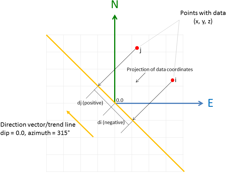
Data point projection on trend line click to enlarge
To create the cross plot, the position of the input data is projected on the calculated trend line. See the figure. The values shown along the horizontal axis of the cross plot indicate the relative position (‘d’ in the figure) of the projected data points on the line. The zero point is just a mathematical point without geographical meaning. The horizontal axis can thus be seen as representing the projection (trend) line, with its azimuth directed towards the right. Although not directly reducible to actual geographical coordinates, the cross plot gives you an idea of the input data distribution with respect to the orientation (azimuth) of the trend line.